This blog post and accompanying code are inspired by this article on Towards Data Science, which walks through extracting dominant image colours using Python.
The challenge
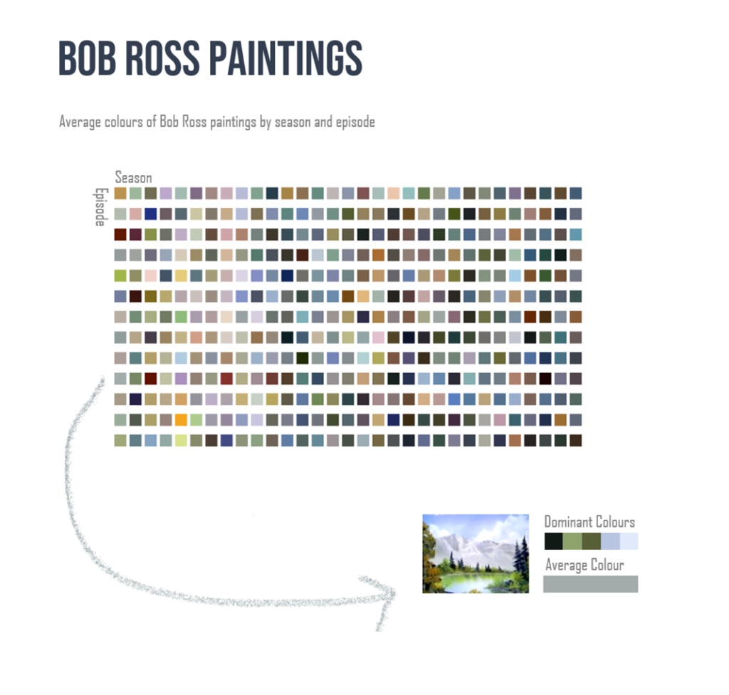
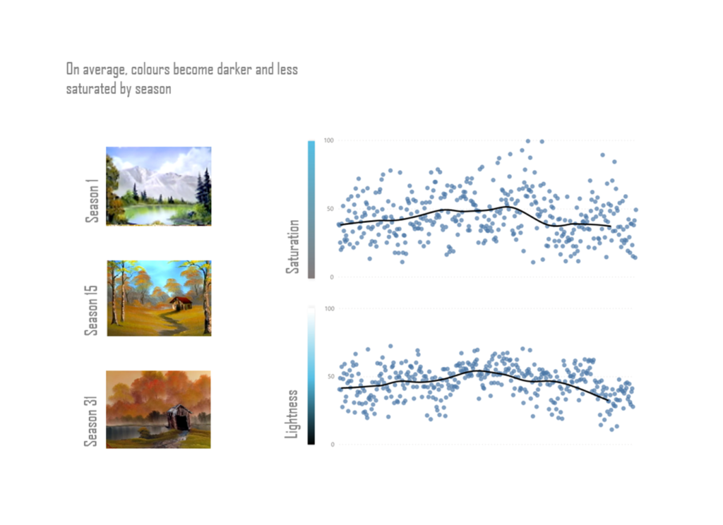
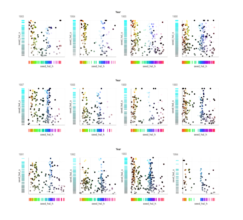
From a Nightgale Data Visualisation challenge using the Bob Ross dataset, the goal was to extract dominant colours from each episode’s painting. These colours were then analysed to find trends, patterns and create visualisations in Power BI.
You can find the PowerPoint presentation of the results here.
A YouTube presentation of the design process can be found here.


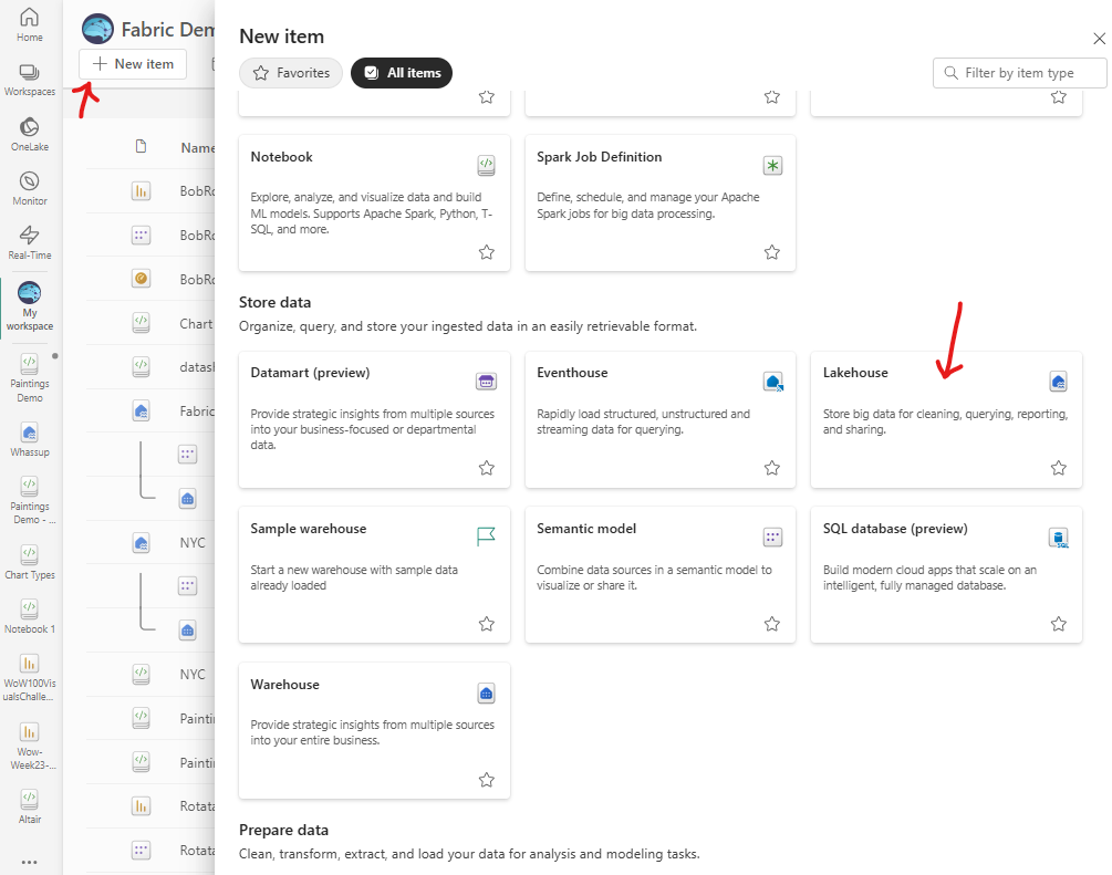
How
- Create new Lakehouse
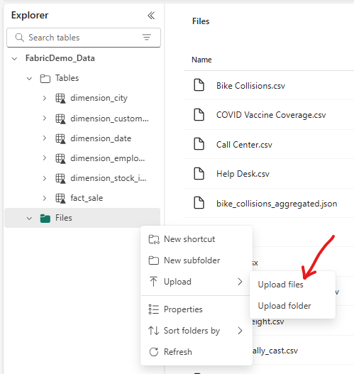
2. Upload the Bob Ross CSV to your Files.
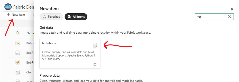
3. With the data saved in your Lakehouse, create a new Notebook and point it to the Lakehouse containing your dataset.

4. Within the Notebook, install the dominant-color-recognizer package.
pip install dominantcolorrecognizer5. Load and display your DataFrame to ensure the data is correctly loaded.
import pandas as pd
df = pd.read_csv("/lakehouse/default/Files/bob_ross_paintings.txt")
print(df)
6. Retrieve an image from a URL for testing.
import urllib.request
from PIL import Image

# Retrieving the resource located at the URL
# and storing it in the file name a.png
url = "https://www.twoinchbrush.com/images/painting156.png"
urllib.request.urlretrieve(url, "painting156.png")

# Opening the image and displaying it (to confirm its presence)
img = Image.open(r"painting156.png")
img.show()
Optional Step: Resize Images
If your images are large, it’s recommended to resize them before extracting colours. This improves performance and reduces processing time.
To resize the images follow the instructions per the Toward Data Science article referenced above.
Extracting Colours
- Extract dominant colours from the image and print the RGB and HEX codes for each colour.
# Get the dominant colors in HEX and RGB format
colors_hex = ColorAnalyzer(HEXColorModel()).get_dominant_colors(image_path, 5)
colors_rgb = ColorAnalyzer(RGBColorModel()).get_dominant_colors(image_path, 5)

print("HEX Colors:", colors_hex)
print("RGB Colors:", colors_rgb)
2. Display dominant colours visually
# Create a new figure for displaying the colors
fig, ax = plt.subplots(figsize=(8, 2))

# Hide the axes
ax.axis('off')

# Number of colors
n_colors = len(colors_hex)

# Display the HEX and RGB colors
for i, (hex_color, rgb_color) in enumerate(zip(colors_hex, colors_rgb)):
    # Create a rectangle for the HEX color
    rect_hex = plt.Rectangle((i, 1), 1, 1, color=hex_color)
    ax.add_patch(rect_hex)

    # Display the HEX value
    ax.text(i + 0.5, 0.5, hex_color, ha='center', va='center', fontsize=12, color='black')

    # Display the RGB value below the HEX value
    ax.text(i + 0.5, -0.5, str(rgb_color), ha='center', va='center', fontsize=12, color='black')

# Set the limits of the plot to make room for the text
ax.set_xlim(0, n_colors)
ax.set_ylim(-1, 2)

plt.show()
To extract dominant colours for images in your DataFrame (rather than just a single static URL), update with the code below.
# Get the first image URL from the "img_src" column
image_url = df.loc[0, "img_src"]  # Change the index if you want a different painting
image_filename = "painting.png"

# Download the image from the URL
urllib.request.urlretrieve(image_url, image_filename)

# Open and display the image
img = Image.open(image_filename)
img.show()
Full code :
# Step 1: Install the required package
%pip install dominantcolorrecognizer

# Step 2: Import necessary libraries
import pandas as pd
import urllib.request
from PIL import Image
import matplotlib.pyplot as plt
import numpy as np
from dominant_color_recognizer import ColorAnalyzer, RGBColorModel, HEXColorModel

# Step 3: Load the CSV file from Fabric Lakehouse
df = pd.read_csv("/lakehouse/default/Files/bob_ross_paintings.txt")
print(df.head())  # Display a preview to verify the structure

# Step 4: Get the first image URL from the "img_src" column
image_url = df.loc[0, "img_src"]  # Change the index if you want a different painting
image_filename = "painting.png"

# Step 5: Download the image from the URL
urllib.request.urlretrieve(image_url, image_filename)

# Step 6: Open and display the image
img = Image.open(image_filename)
img.show()

# Step 7: Analyze the image for dominant colors
# Load and display the original image
image = Image.open(image_filename)

# Display the original image
plt.figure(figsize=(5, 5))
plt.imshow(image)
plt.axis('off')
plt.title('Original Image')
plt.show()

# Get the dominant colors in HEX and RGB format
colors_hex = ColorAnalyzer(HEXColorModel()).get_dominant_colors(image_filename, 5)
colors_rgb = ColorAnalyzer(RGBColorModel()).get_dominant_colors(image_filename, 5)

print("HEX Colors:", colors_hex)
print("RGB Colors:", colors_rgb)

# Step 8: Display the dominant colors
fig, ax = plt.subplots(figsize=(8, 2))
ax.axis('off')

n_colors = len(colors_hex)

for i, (hex_color, rgb_color) in enumerate(zip(colors_hex, colors_rgb)):
    rect_hex = plt.Rectangle((i, 1), 1, 1, color=hex_color)
    ax.add_patch(rect_hex)
    ax.text(i + 0.5, 0.5, hex_color, ha='center', va='center', fontsize=12, color='black')
    ax.text(i + 0.5, -0.5, str(rgb_color), ha='center', va='center', fontsize=12, color='black')

ax.set_xlim(0, n_colors)
ax.set_ylim(-1, 2)
plt.show()
Automating the Process
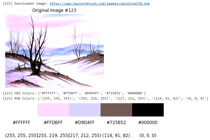
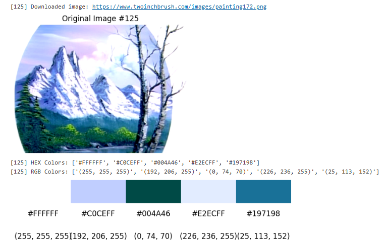
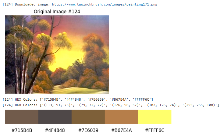
To dynamically pull dominant colours for all images in your DataFrame, use the provided loop code
# Step 1: Install the required package
# pip install dominantcolorrecognizer

# Step 2: Import necessary libraries
import pandas as pd
import urllib.request
from PIL import Image
import matplotlib.pyplot as plt
import numpy as np
from dominant_color_recognizer import ColorAnalyzer, RGBColorModel, HEXColorModel

# Step 3: Load the CSV file from Fabric Lakehouse
df = pd.read_csv("/lakehouse/default/Files/bob_ross_paintings.txt")
print(f"Found {len(df)} paintings")

# Step 4: Loop through all image URLs in the DataFrame
for index, row in df.iterrows():
    image_url = row["img_src"]  # Make sure this matches your column name
    image_filename = f"painting_{index}.png"

    try:
        # Download the image
        urllib.request.urlretrieve(image_url, image_filename)
        print(f"[{index}] Downloaded image: {image_url}")

        # Open the image
        image = Image.open(image_filename)

        # Display the original image
        plt.figure(figsize=(5, 5))
        plt.imshow(image)
        plt.axis('off')
        plt.title(f'Original Image #{index}')
        plt.show()

        # Get the dominant colors
        colors_hex = ColorAnalyzer(HEXColorModel()).get_dominant_colors(image_filename, 5)
        colors_rgb = ColorAnalyzer(RGBColorModel()).get_dominant_colors(image_filename, 5)

        print(f"[{index}] HEX Colors: {colors_hex}")
        print(f"[{index}] RGB Colors: {colors_rgb}")

        # Display the dominant colors
        fig, ax = plt.subplots(figsize=(8, 2))
        ax.axis('off')

        for i, (hex_color, rgb_color) in enumerate(zip(colors_hex, colors_rgb)):
            rect_hex = plt.Rectangle((i, 1), 1, 1, color=hex_color)
            ax.add_patch(rect_hex)
            ax.text(i + 0.5, 0.5, hex_color, ha='center', va='center', fontsize=12, color='black')
            ax.text(i + 0.5, -0.5, str(rgb_color), ha='center', va='center', fontsize=12, color='black')

        ax.set_xlim(0, len(colors_hex))
        ax.set_ylim(-1, 2)
        plt.show()

    except Exception as e:
        print(f"[{index}] Failed to process image: {image_url}")
        print("Error:", e)

Adding the dominant colours to your Lakehouse
To loop through and add the dominant colours to the dataframe then save as a new CSV file to your Lakehouse:
# pip install dominantcolorrecognizer

import pandas as pd
import urllib.request
from PIL import Image
from dominant_color_recognizer import ColorAnalyzer, RGBColorModel, HEXColorModel
import os

# Load the original CSV
df = pd.read_csv("/lakehouse/default/Files/bob_ross_paintings.txt")

# Prepare analyzer instances
hex_analyzer = ColorAnalyzer(HEXColorModel())
rgb_analyzer = ColorAnalyzer(RGBColorModel())

# Create a list to collect results
results = []

# Make a temp folder to store downloaded images
os.makedirs("temp_images", exist_ok=True)

# Process each image
for index, row in df.iterrows():
    image_url = row["img_src"]  # Make sure column name is correct
    image_filename = f"temp_images/painting_{index}.png"

    try:
        # Download image
        urllib.request.urlretrieve(image_url, image_filename)

        # Get dominant colors
        colors_hex = hex_analyzer.get_dominant_colors(image_filename, 5)
        colors_rgb = rgb_analyzer.get_dominant_colors(image_filename, 5)

        # Store results in a dict (flattened)
        result = {
            "index": index,
            "image_url": image_url,
            "hex_1": colors_hex[0], "hex_2": colors_hex[1], "hex_3": colors_hex[2],
            "hex_4": colors_hex[3], "hex_5": colors_hex[4],
            "rgb_1": str(colors_rgb[0]), "rgb_2": str(colors_rgb[1]), "rgb_3": str(colors_rgb[2]),
            "rgb_4": str(colors_rgb[3]), "rgb_5": str(colors_rgb[4])
        }

        results.append(result)

    except Exception as e:
        print(f"[{index}] Failed: {image_url} — {e}")
        continue

# Convert results into a DataFrame
results_df = pd.DataFrame(results)

# Save to new CSV file in Fabric Lakehouse
output_path = "/lakehouse/default/Files/bob_ross_dominant_colors.csv"
results_df.to_csv(output_path, index=False)

print(f"Complete. Saved dominant colors for {len(results_df)} paintings to: {output_path}")
Note: Running this on unresized images significantly increases processing time and notebook size. In one test, this process took 21 minutes and 51 seconds.
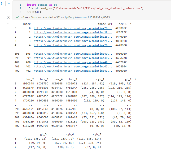
Verifying the Data
Once your CSV is loaded, do a quick check to confirm that the data appears as expected:
Connect to dataset in Power BI
There are multiples ways of connecting Power BI to your Lakehouse data.
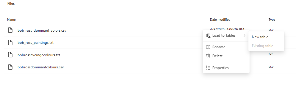
One of the simpler ways is to navigate to your Lakehouse, selecting the ellipsis on the newly created csv > Load to Tables > New Table
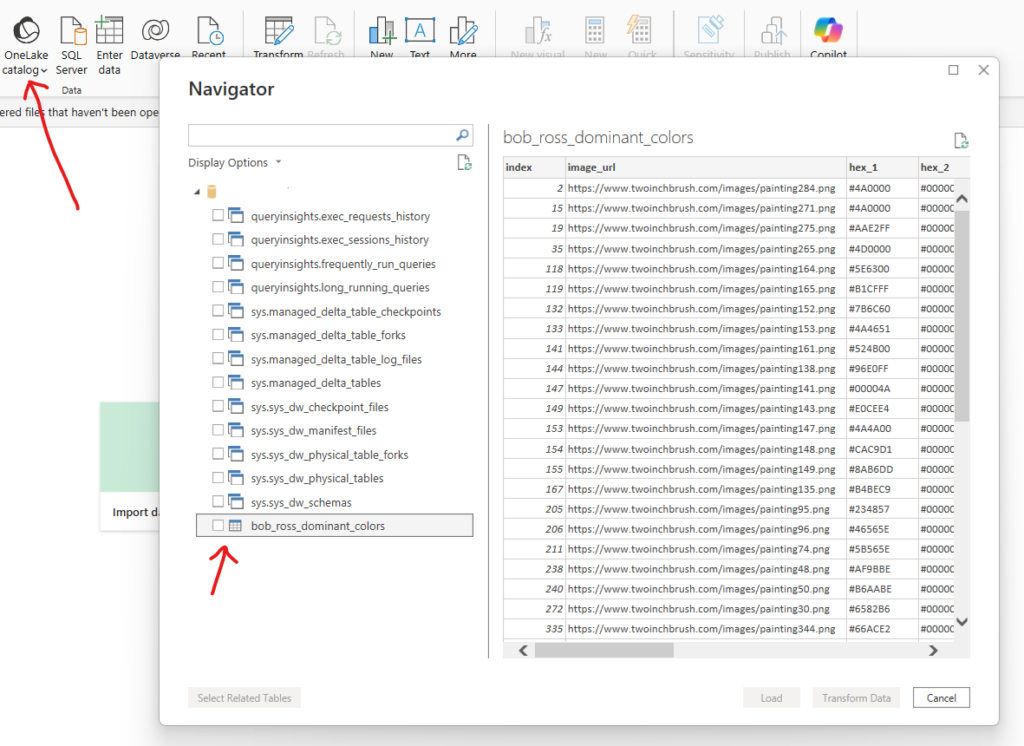
From Power BI Desktop ribbon, select OneLake catalog > (Your Lakehouse) > Connect, and select the relevant Table