Images and custom shapes in Deneb

Over the past few months, I’ve had considerable fun exploring images and custom shapes with Deneb Custom visual for Power BI. I’ve finally gotten around to blogging about it.

There are some cool techniques I learned along the way such as changing the scales of trail marks, clipping point marks, using multiple datasets and performing transformations on these datasets within the Deneb Editor.

Images

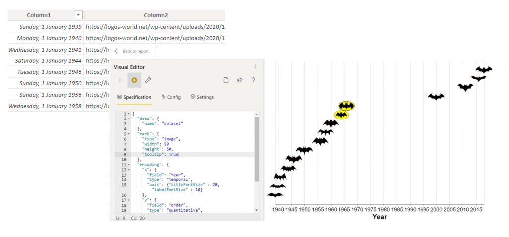
The following chart uses images as series labels:

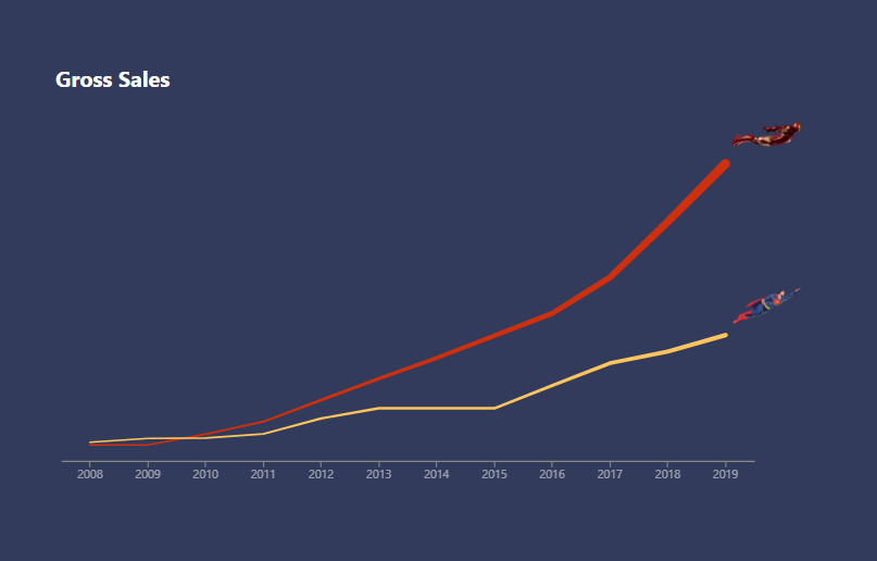
The dataset is simple and contains the following fields:

I used trail marks for the cumulative totals.

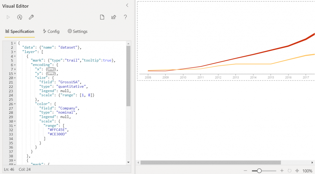
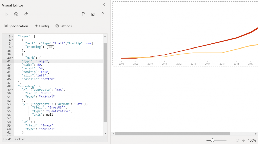
Then layered an image mark with width and height of 50.

In the encoding channels I found the last point of the series using argmax and for the image URL I referenced the “Image” field.

With the standalone Deneb visual I am able to use image web URLs as I had done with this scatterplot last year:

However, this feature is not available in the AppSource Certified version of Deneb due to restrictions in the certification process. To have the image marks appear in the Certified version of Deneb I would need to convert the images to Base64.

Base64 strings can be stored in Power BI datasets however, there are limitations on the string size as noted in Chris Webb’s blog <here>.

The images I had were both approx 150kb and exceeded the string length upon conversion. I could have found smaller images or followed Chris’ excellent instructions to achieve the result I wanted.

But. I wouldn’t be learning anything new.

Instead, I wanted to test the visual and explore alternative methods to see if they could work – useful knowledge for future projects.

I found that I could paste Base64 strings directly into the visual editor. There was a noticeable but still perfectly tolerable lag.

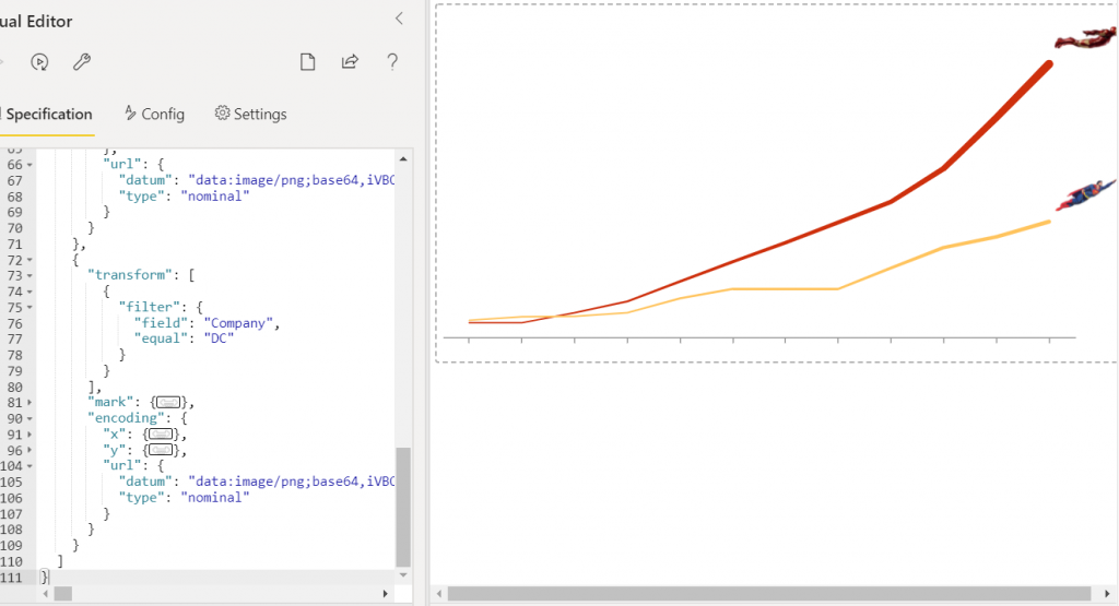
Method 1: Create two separate mark layers

In this version, I created a layer for each image and filtered the dataset ‘Company’ = ‘DC’ or ‘Company’ = ‘Marvel’. I changed the URL reference from ‘field’ to ‘datum’ and pasted the Base64 in.

Method 2 : Lookup a second manual dataset

In this version, I pasted a second manual dataset in the form of:

"datasets": {
   "dataset2": [
   {"Company": "CompanyName1", "img": "Base64String1"},
   {"Company": "CompanyName2", "img": "Base64String2"}
   ]
}

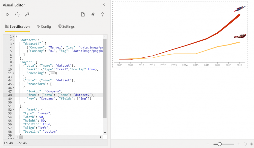
When then made sure each layer referenced the correct dataset:

“data”: {“name”: “dataset”} for the Power BI dataset

“data”: {“name”: “dataset2”} for the manually entered dataset.

Within the image mark layer I referenced the Power BI dataset and transformed it to add the Base64 images of the second dataset by using a lookup function:

{
      "data": {"name": "dataset"},
      "transform": [
        {
          "lookup": "Company",
          "from": {
            "data": {
              "name": "dataset2"
            },
            "key": "Company",
            "fields": ["img"]
          }
        }
      ]...
}

Full structure below (Base64 strings removed for brevity):

{
  "datasets": {
    "dataset2": [
      {
        "Company": "Marvel",
        "img": "data:image/png;base64"
      },
      {
        "Company": "DC",
		"img": "data:image/png;base64"
      }
    ]
  },
  "layer": [
    {
      "data": {"name": "dataset"},
      "mark": {
        "type": "trail",
        "tooltip": true
      },
      "encoding": {
        "x": {
          "field": "Date",
          "type": "ordinal",
          "axis": {
            "title": "",
            "labelAngle": 0
          }
        },
        "y": {
          "field": "GrossUSA",
          "type": "quantitative",
          "axis": null
        },
        "size": {
          "field": "GrossUSA",
          "type": "quantitative",
          "legend": null,
          "scale": {"range": [1, 8]}
        },
        "color": {
          "field": "Company",
          "type": "nominal",
          "legend": null,
          "scale": {
            "range": [
              "#FFC45E",
              "#CE300D"
            ]
          }
        }
      }
    },
    {
      "data": {"name": "dataset"},
      "transform": [
        {
          "lookup": "Company",
          "from": {
            "data": {
              "name": "dataset2"
            },
            "key": "Company",
            "fields": ["img"]
          }
        }
      ],
      "mark": {
        "type": "image",
        "width": 50,
        "height": 50,
        "tooltip": true,
        "align": "left",
        "baseline": "bottom"
      },
      "encoding": {
        "x": {
          "aggregate": "max",
          "field": "Date",
          "type": "ordinal"
        },
        "y": {
          "aggregate": {
            "argmax": "Date"
          },
          "field": "GrossUSA",
          "type": "quantitative",
          "axis": null
        },
        "url": {
          "field": "img",
          "type": "nominal"
        }
      }
    }
  ]
}

Shapes

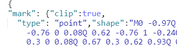
Another feature of Vega and Vega-Lite is custom shapes for point marks.

These take the form of SVG paths.

Vega only needs the path coordinates, which everything between these quotation marks.

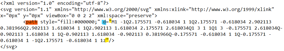
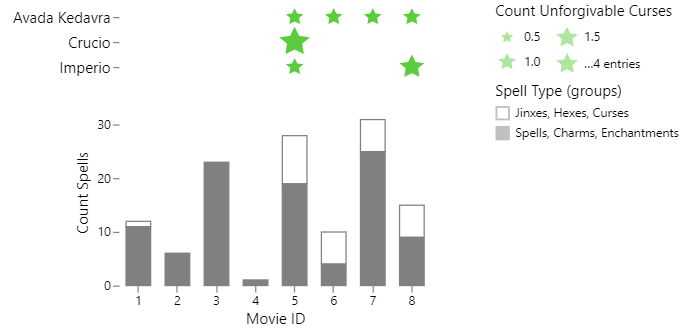
Here I used a path for a star shape:

"mark": {
    "type": "point",
    "shape": "M0,.5L.6,.8L.5,.1L1,-.3L.3,-.4L0,-1L-.3,-.4L-1,-.3L-.5,.1L-.6,.8L0,.5Z",
    "filled": true,
    "color":"#5bcd3d",
    "tooltip": true
  },

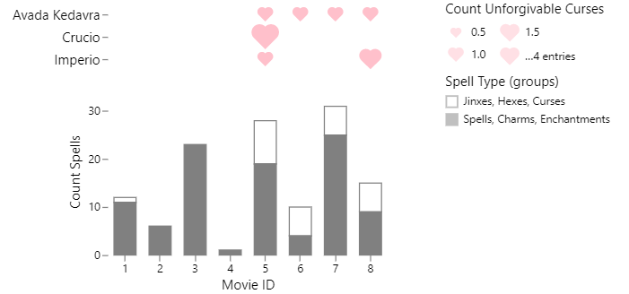
Which can be switched out for a heart shape:

"mark": {
    "type": "point",
    "shape": "M.83.09,0,.91-.83.09a.59.59,0,0,1,0-.83A.59.59,0,0,1,0-.74a.59.59,0,0,1,.83,0A.59.59,0,0,1,.83.09Z",
    "filled": true,
    "color":"#5bcd3d",
    "tooltip": true
  },

This enables me to get really silly and do odd things like this:

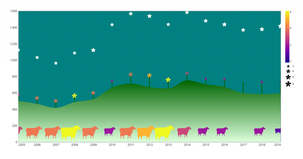
The sheep were “clipped” to stop them going over the bounds of the chart.

To create the shapes I needed to find or draw a simple SVG icon (a single shape with no clip paths), copy this into Adobe Illustrator and resize to 2x2px, centre the image to 0,0px.

Edit: This is because according to the Vega-lite documentation, for correct sizing, the paths should be defined within a square bounding box (viewbox) with coordinates ranging from -1 to 1. This ensures the point is plotted at its centre. More information on SVGs here.

Obtaining the paths was quite fiddly. Export or Save As SVG would not work as the viewbox would always recalibrate to 0 0 2 2. To keep the SVG path as I needed it, within a viewbox of -1 -1 1 1, I would have to select the object, select copy and then paste into a notepad and extract the path from there.